This short how-to guides you through the steps to create a timeseries of the population using GHS Population data and save it as a csv file. The final csv file can be used as, e.g., exposure data for the drought risk estimation.
We demonstrate the use of two datasets from the Global Human Settlement (GHS) project:
GHS-POP: Historical and projected population (1975-2030), GHS Population Grid. Find more info in Schiavina et al. (2023) and Pesaresi et al. (2024).
GHS-WUP-POP: Urban population projections (1975-2100), GHS WUP Population. Find more info in Schiavina et al. (2025) and Jacobs-Crisioni & others (2025).
Settings
User settings
admin_id = "ITF2"  # Example admin ID for Central Greece

# Set working directory
workdir = "/etc/ecmwf/nfs/dh2_home_a/nejk/code/extreme_precip_exposure"

# Choose dataset: 'GHS_POP' (1975-2030) or 'GHS_WUP_POP' (1975-2100)
dataset_choice = "GHS_POP"  # Change to "GHS_WUP_POP" for urban population projections
Setup of environment
import xarray as xr
import numpy as np
import pandas as pd
import matplotlib.pyplot as plt
import geopandas as gpd
import regionmask
from pathlib import Path
import rioxarray as rxr
import os
import re

# Set working directoy
os.chdir(workdir)
print(f"Working directory: {os.getcwd()}")

# Set up data directories
data_dir = Path("./data")
ghs_pop_dir = data_dir / "population" / "GHS_POP"
ghs_wup_dir = data_dir / "population" / "GHS_WUP_POP"

# Set directory and file pattern based on dataset choice
if dataset_choice == "GHS_POP":
    ghs_dir = ghs_pop_dir
    file_pattern = "*/GHS_POP_E*_GLOBE_R2023A_4326_30ss_V1_0.tif"
    dataset_name = "GHS-POP"
    year_range = "(1975-2030)"
elif dataset_choice == "GHS_WUP_POP":
    ghs_dir = ghs_wup_dir
    file_pattern = "*/GHS_WUP_POP_E*_GLOBE_R2025A_4326_30ss_V1_0.tif"
    dataset_name = "GHS-WUP"
    year_range = "(1975-2100)"
else:
    raise ValueError(f"Invalid dataset_choice: {dataset_choice}. Must be 'GHS_POP' or 'GHS_WUP_POP'")

print(f"\nSelected dataset: {dataset_name} {year_range}")
print(f"Data directory: {ghs_dir}")
Working directory: /etc/ecmwf/nfs/dh2_home_a/nejk/code/extreme_precip_exposure
Selected dataset: GHS-POP (1975-2030)
Data directory: data/population/GHS_POP
Setup region specifics
# Read NUTS shapefiles
regions_dir = data_dir / 'regions'
nuts_shp = regions_dir / 'NUTS_RG_20M_2024_4326' / 'NUTS_RG_20M_2024_4326.shp'
nuts_gdf = gpd.read_file(nuts_shp)

# Select the region of interest
sel_gdf = nuts_gdf[nuts_gdf['NUTS_ID'] == admin_id]
print(f"Found {admin_id} region: {sel_gdf['NUTS_NAME'].values[0]}")
print(f"Bounding box: {sel_gdf.geometry.total_bounds}")
lon_min, lat_min, lon_max, lat_max = sel_gdf.geometry.total_bounds

# Create a regionmask from the admin region geometry
admin_mask = regionmask.from_geopandas(sel_gdf, names='NUTS_ID')
Found ITF2 region: Molise
Bounding box: [13.94103834 41.38256335 15.13817868 42.07005936]
Download Exposure Data
The data is downloaded manually through the following webpage: https://
We download the global data for all years available, but at 30 arcsec resolution, and in the WGS84 (or EPSG: 4326) projection for easier handling of the data afterwards. The images below show the web interface to download the datasets and detail the settings used.
| Download GHS population | Download GHS WUP population |
|---|---|
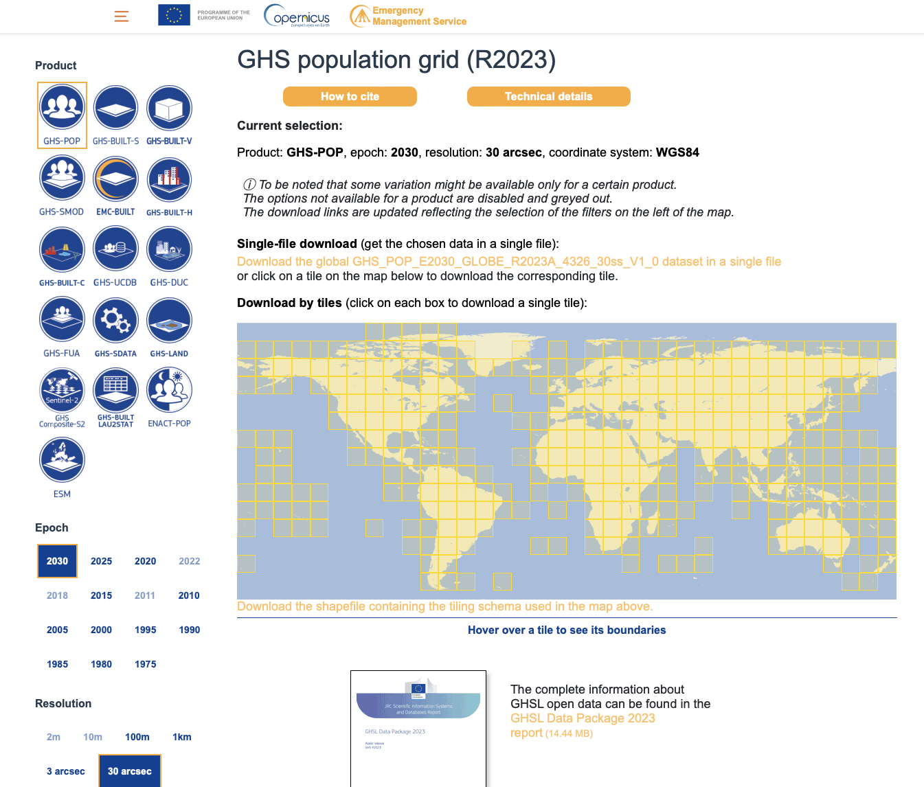 |  |
GHS-POP (1975-2030): Download files named GHS_POP_E{YYYY}_GLOBE_R2023A_4326_30ss_V1_0.tif for years 1975, 1980, 1985, 1990, 1995, 2000, 2005, 2010, 2015, 2020, 2025, 2030.
GHS-WUP (1975-2100): Download files named GHS_WUP_POP_E{YYYY}_GLOBE_R2025A_4326_30ss_V1_0.tif for years from 1975 to 2100 in 5-year intervals.
Once downloaded, move these files into the following subdirectory structure:
./data/population/GHS_POP/for GHS-POP files./data/population/GHS_WUP_POP/for GHS-WUP files
Process Population Data
Read global data
# List all GHS tif files based on selected dataset
ghs_files = sorted(list(ghs_dir.glob(file_pattern)))
print(f"Found {len(ghs_files)} {dataset_name} files:")
for f in ghs_files:
    print(f"  {f.name}")
Found 12 GHS-POP files:
GHS_POP_E1975_GLOBE_R2023A_4326_30ss_V1_0.tif
GHS_POP_E1980_GLOBE_R2023A_4326_30ss_V1_0.tif
GHS_POP_E1985_GLOBE_R2023A_4326_30ss_V1_0.tif
GHS_POP_E1990_GLOBE_R2023A_4326_30ss_V1_0.tif
GHS_POP_E1995_GLOBE_R2023A_4326_30ss_V1_0.tif
GHS_POP_E2000_GLOBE_R2023A_4326_30ss_V1_0.tif
GHS_POP_E2005_GLOBE_R2023A_4326_30ss_V1_0.tif
GHS_POP_E2010_GLOBE_R2023A_4326_30ss_V1_0.tif
GHS_POP_E2015_GLOBE_R2023A_4326_30ss_V1_0.tif
GHS_POP_E2020_GLOBE_R2023A_4326_30ss_V1_0.tif
GHS_POP_E2025_GLOBE_R2023A_4326_30ss_V1_0.tif
GHS_POP_E2030_GLOBE_R2023A_4326_30ss_V1_0.tif
# Read all GHS files and extract years (clipped to region bounding box)
datasets = []
years = []

for tif_file in ghs_files:
    # Read using rioxarray
    ds = rxr.open_rasterio(tif_file)

    # Clip using sel() instead of rio.clip_box to avoid artifacts
    # Note: y coordinates are typically in descending order in raster data
    ds_clipped = ds.sel(
        x=slice(lon_min, lon_max),
        y=slice(lat_max, lat_min)  # Note: reversed for descending y-coords
    )

    # Extract year from filename (looking for pattern E{YYYY})
    year_match = re.search(r'E(\d{4})', tif_file.name)
    if year_match:
        year = int(year_match.group(1))
        years.append(year)
        print(f"Processing year: {year}")
    else:
        print(f"Warning: Could not extract year from {tif_file.name}")
        continue

    datasets.append(ds_clipped)

# Sort datasets and years together by year
sorted_pairs = sorted(zip(years, datasets), key=lambda x: x[0])
years, datasets = zip(*sorted_pairs)

# Concatenate along new time dimension
pop_ds = xr.concat(datasets, dim="time")
pop_ds = pop_ds.rename("population")
pop_ds = pop_ds.squeeze("band", drop=True)

# Assign time based on extracted years
pop_ds["time"] = pd.to_datetime([f"{year}-01-01" for year in years])
pop_ds = pop_ds.assign_coords(time=pop_ds.time)

# Replace potential fill values with NaN (common fill values: -200, -99999, etc.)
pop_ds = pop_ds.where(pop_ds >= 0)

print(f"\n{dataset_name} dataset shape: {pop_ds.shape}")
print(f"Years available: {years}")
print(f"Coordinate ranges: x=[{float(pop_ds.x.min()):.2f}, {float(pop_ds.x.max()):.2f}], y=[{float(pop_ds.y.min()):.2f}, {float(pop_ds.y.max()):.2f}]")
print(f"Data value range: [{float(pop_ds.min()):.2f}, {float(pop_ds.max()):.2f}]")
Processing year: 1975
Processing year: 1980
Processing year: 1985
Processing year: 1990
Processing year: 1995
Processing year: 2000
Processing year: 2005
Processing year: 2010
Processing year: 2015
Processing year: 2020
Processing year: 2025
Processing year: 2030
/etc/ecmwf/ssd/ssd1/jupyterhub/nejk-jupyterhub/tmpdirs/nejk.15156925/ipykernel_3177436/1759060448.py:33: FutureWarning: In a future version of xarray the default value for join will change from join='outer' to join='exact'. This change will result in the following ValueError: cannot be aligned with join='exact' because index/labels/sizes are not equal along these coordinates (dimensions): 'x' ('x',) The recommendation is to set join explicitly for this case.
  pop_ds = xr.concat(datasets, dim="time")
/etc/ecmwf/ssd/ssd1/jupyterhub/nejk-jupyterhub/tmpdirs/nejk.15156925/ipykernel_3177436/1759060448.py:33: FutureWarning: In a future version of xarray the default value for join will change from join='outer' to join='exact'. This change will result in the following ValueError: cannot be aligned with join='exact' because index/labels/sizes are not equal along these coordinates (dimensions): 'y' ('y',) The recommendation is to set join explicitly for this case.
  pop_ds = xr.concat(datasets, dim="time")
GHS-POP dataset shape: (12, 246, 432)
Years available: (1975, 1980, 1985, 1990, 1995, 2000, 2005, 2010, 2015, 2020, 2025, 2030)
Coordinate ranges: x=[13.95, 15.14], y=[41.39, 42.06]
Data value range: [0.00, 5587.87]
Extract regional data
# Data is already clipped to bounding box, so we use it directly as pop_region
pop_region = pop_ds

# Create admin region mask
pop_admin_mask_raw = admin_mask.mask(pop_region.x, pop_region.y)
pop_admin_mask = xr.DataArray(
    (~np.isnan(pop_admin_mask_raw.values)).astype(float),
    coords={'y': pop_region.y, 'x': pop_region.x},
    dims=['y', 'x']
)

print(f"{dataset_name} admin mask: {pop_admin_mask.sum().values:.0f} grid cells")
GHS-POP admin mask: 62757 grid cells
# Diagnostic: Check data quality
print("Data diagnostics:")
print(f"  Population grid shape: {pop_region.shape}")
print(f"  Mask shape: {pop_admin_mask.shape}")
print(f"  Number of masked cells: {pop_admin_mask.sum().values:.0f}")
print(f"  Population data - NaN count: {pop_region.isnull().sum().values}")
print(f"  Population data - Valid values: {(~pop_region.isnull()).sum(['x', 'y']).values}")

# Check a single time slice
sample_time = 0
sample_data = pop_region.isel(time=sample_time)
print(f"\nSample year {pop_region.time.dt.year.values[sample_time]}:")
print(f"  Valid cells (not NaN): {(~sample_data.isnull()).sum().values}")
print(f"  Min value: {float(sample_data.min()):.2f}")
print(f"  Max value: {float(sample_data.max()):.2f}")
print(f"  Mean value: {float(sample_data.mean()):.2f}")
Data diagnostics:
Population grid shape: (12, 246, 432)
Mask shape: (246, 432)
Number of masked cells: 62757
Population data - NaN count: 1133568
Population data - Valid values: [11808 11808 11808 11808 11808 11808 11808 11808 11808 11808 11808 11808]
Sample year 1975:
Valid cells (not NaN): 11808
Min value: 0.00
Max value: 5587.87
Mean value: 41.27
Calculate total population
We calculate the total population within the region by summing all population values within the masked area.
# Calculate total population for each year
pop_results = []

for i, year in enumerate(years):
    # Get data for this year
    data = pop_region.isel(time=i)

    # Apply mask and sum population
    masked_data = data.where(pop_admin_mask == 1, 0)
    total_pop = masked_data.sum().values

    pop_results.append({
        'year': year,
        'population': total_pop
    })

    print(f"{year}: {total_pop:,.0f} people")

df_pop = pd.DataFrame(pop_results)
print(f"\n{dataset_name} results:")
print(df_pop)
1975: 324,997 people
1980: 322,793 people
1985: 315,149 people
1990: 307,101 people
1995: 300,027 people
2000: 292,010 people
2005: 290,995 people
2010: 291,741 people
2015: 277,825 people
2020: 254,974 people
2025: 236,998 people
2030: 219,359 people
GHS-POP results:
year population
0 1975 324997.08408640954
1 1980 322792.68684490526
2 1985 315148.6960769107
3 1990 307101.3803042464
4 1995 300026.7435338818
5 2000 292010.40850526845
6 2005 290995.1234416002
7 2010 291740.6890532695
8 2015 277824.9303738809
9 2020 254973.71546023677
10 2025 236997.88262077374
11 2030 219358.9062808804
Save Regional Population Data
Save results to CSV
# Create output directory
output_dir = data_dir / admin_id / "ghs_population"
output_dir.mkdir(parents=True, exist_ok=True)

# Save results with dataset-specific filename
dataset_suffix = "ghs_pop" if dataset_choice == "GHS_POP" else "ghs_wup"
csv_file = output_dir / f"population_{dataset_suffix}_{admin_id}.csv"
df_pop.to_csv(csv_file, index=False)
print(f"Saved {dataset_name} results to: {csv_file}")
Saved GHS-POP results to: data/ITF2/ghs_population/population_ghs_pop_ITF2.csv
Output summary
Output files created:
population_ghs_pop_{admin_id}.csv- Population timeseries (1975-2030) from GHS-POPpopulation_ghs_wup_{admin_id}.csv- Population timeseries (1975-2100) from GHS-WUP
These CSV files can now be used as exposure data in drought risk assessments or other analyses.
- Schiavina, M., Freire, S., Carioli, A., & MacManus, K. (2023). GHS-POP R2023A – GHS population grid multitemporal (1975-2030) [Data set]. European Commission, Joint Research Centre (JRC). 10.2905/2FF68A52-5B5B-4A22-8F40-C41DA8332CFE
- Pesaresi, M., Schiavina, M., Politis, P., Freire, S., Krasnodębska, K., Uhl, J. H., Carioli, A., Corbane, C., Dijkstra, L., Florio, P., Friedrich, H. K., Gao, J., Leyk, S., Lu, L., Maffenini, L., Mari-Rivero, I., Melchiorri, M., Syrris, V., Van Den Hoek, J., & Kemper, T. (2024). Advances on the Global Human Settlement Layer by joint assessment of Earth Observation and population survey data. International Journal of Digital Earth, 17(1). 10.1080/17538947.2024.2390454
- Schiavina, M., Freire, S., Carioli, A., MacManus, K., Jacobs-Crisioni, C., Claassens, J., Hilferink, M., & Dijkstra, L. (2025). GHS-WUP-POP R2025A – GHS-WUP population spatial raster dataset, derived from GHS-POP (R2023) and projected using the CRISP model, multitemporal (1975-2100) [Data set]. European Commission, Joint Research Centre (JRC). 10.2905/adba95af-db56-4569-acd3-9513201eba30
- Jacobs-Crisioni, C., & others. (2025). Population projections by degree of urbanisation for the UN World Urbanization Prospects: introducing the CRISP model [Techreport]. Publications Office of the European Union. 10.2760/7163875