In this tutorial, we combine drought hazard (duration) with population data to estimate the number of people exposed to drought in Central Greece (NUTS2 region EL64). Exposure is a key component of drought risk assessment.
Setup
import pandas as pd
import matplotlib.pyplot as plt
import numpy as np
import os
from pathlib import Path

# Configure plotting
plt.rcParams['figure.figsize'] = (12, 6)
plt.rcParams['font.size'] = 11
Settings
# Configuration
admin_id = 'EL64'

# Reference period (WMO standard: 1991-2020)
baseline_start = 1991
baseline_end = 2020

# Paths
data_dir = Path(f'data/{admin_id}')

# Load preprocessed data
drought_reanalysis = data_dir / 'drought_hazard' / f'drought_duration_reanalysis_{admin_id}.csv'
drought_proj = data_dir / 'drought_hazard' / f'drought_duration_projections_{admin_id}.csv'
population_wup = data_dir / 'ghs_population' / f'population_ghs_wup_{admin_id}.csv'

print(f"Region: {admin_id} (Central Greece)")
print(f"\nData files:")
print(f"  Drought (reanalysis): {drought_reanalysis.name}")
print(f"  Drought (projections): {drought_proj.name}")
print(f"  Population: {population_wup.name}")
Region: EL64 (Central Greece)
Data files:
Drought (reanalysis): drought_duration_reanalysis_EL64.csv
Drought (projections): drought_duration_projections_EL64.csv
Population: population_ghs_wup_EL64.csv
Load Data
# Load drought reanalysis data
drought_hist_df = pd.read_csv(drought_reanalysis)
drought_hist_df['time'] = pd.to_datetime(drought_hist_df['time'])
drought_hist_df['year'] = drought_hist_df['time'].dt.year

# Load drought projection data
drought_proj_df = pd.read_csv(drought_proj)
drought_proj_df['time'] = pd.to_datetime(drought_proj_df['time'])
drought_proj_df['year'] = drought_proj_df['time'].dt.year

# Load population data (GHS-WUP: 1975-2100)
pop_df = pd.read_csv(population_wup)

# Fill gaps in population timeseries using persistence (forward fill)
# Create complete year range from drought data
all_years_hist = pd.DataFrame({'year': range(drought_hist_df['year'].min(), drought_hist_df['year'].max() + 1)})
all_years_proj = pd.DataFrame({'year': range(drought_proj_df['year'].min(), drought_proj_df['year'].max() + 1)})
all_years = pd.concat([all_years_hist, all_years_proj]).drop_duplicates().sort_values('year').reset_index(drop=True)

# Merge with population and forward fill missing values
pop_df_filled = all_years.merge(pop_df, on='year', how='left')
pop_df_filled['population'] = pop_df_filled['population'].ffill()

print(f"Drought reanalysis: {drought_hist_df['year'].min()}-{drought_hist_df['year'].max()}")
print(f"Drought projections: {drought_proj_df['year'].min()}-{drought_proj_df['year'].max()}")
print(f"Population (original): {int(pop_df['year'].min())}-{int(pop_df['year'].max())} ({len(pop_df)} years)")
print(f"Population (filled): {int(pop_df_filled['year'].min())}-{int(pop_df_filled['year'].max())} ({len(pop_df_filled)} years)")
print(f"\nClimate models: {drought_proj_df['model'].nunique()}")
print(f"Scenarios: {sorted(drought_proj_df['scenario'].unique())}")

# Use filled population data for all subsequent calculations
pop_df = pop_df_filled
Drought reanalysis: 1940-2023
Drought projections: 1950-2100
Population (original): 1975-2100 (26 years)
Population (filled): 1940-2100 (161 years)
Climate models: 18
Scenarios: ['RCP4_5', 'RCP8_5']
Part 1: Historical Drought Exposure (1975-2020)
We calculate historical drought exposure by combining:
Drought duration from ERA5 reanalysis (observed climate)
Population from GHS-WUP (urban population)
# Merge historical drought with population data
hist_exposure = drought_hist_df[['year', 'dmd']].merge(pop_df_filled, on='year', how='inner')

# Calculate exposure (person-months of drought exposure per year)
hist_exposure['exposure'] = hist_exposure['dmd'] * hist_exposure['population']

print(f"Historical exposure data: {hist_exposure['year'].min()}-{hist_exposure['year'].max()}")
hist_exposure.head()
Historical exposure data: 1940-2023
# Visualize historical exposure components
fig, axes = plt.subplots(3, 1, figsize=(14, 12), sharex=True)

# Panel 1: Drought Duration
axes[0].plot(hist_exposure['year'], hist_exposure['dmd'],
             color='#D62828', linewidth=2, marker='o', markersize=3)
axes[0].set_ylabel('Drought duration\n(months/year)', fontsize=11)
axes[0].set_title('Historical Drought Exposure Components - Central Greece (EL64)',
                  fontsize=14, fontweight='bold', pad=15)
axes[0].grid(True, alpha=0.3, linestyle='--', linewidth=0.5)
axes[0].spines['top'].set_visible(False)
axes[0].spines['right'].set_visible(False)

# Panel 2: Population
axes[1].plot(hist_exposure['year'], hist_exposure['population']/1e6,
             color='#003049', linewidth=2, marker='s', markersize=3)
axes[1].set_ylabel('Population\n(millions)', fontsize=11)
axes[1].grid(True, alpha=0.3, linestyle='--', linewidth=0.5)
axes[1].spines['top'].set_visible(False)
axes[1].spines['right'].set_visible(False)

# Panel 3: Drought Exposure
axes[2].fill_between(hist_exposure['year'], 0, hist_exposure['exposure']/1e6,
                     color='#F77F00', alpha=0.6)
axes[2].plot(hist_exposure['year'], hist_exposure['exposure']/1e6,
             color='#F77F00', linewidth=2)
axes[2].set_ylabel('Drought exposure\n(million person-months/year)', fontsize=11)
axes[2].set_xlabel('Year', fontsize=12)
axes[2].grid(True, alpha=0.3, linestyle='--', linewidth=0.5)
axes[2].spines['top'].set_visible(False)
axes[2].spines['right'].set_visible(False)

plt.tight_layout()
plt.show()

# Calculate baseline statistics
baseline_hist = hist_exposure[
    hist_exposure['year'].between(baseline_start, baseline_end)
]

print(f"\nHistorical baseline ({baseline_start}-{baseline_end}):")
print(f"  Average drought duration: {baseline_hist['dmd'].mean():.2f} months/year")
print(f"  Average population: {baseline_hist['population'].mean()/1e6:.2f} million")
print(f"  Average exposure: {baseline_hist['exposure'].mean()/1e6:.2f} million person-months/year")
Historical baseline (1991-2020):
  Average drought duration: 1.25 months/year
  Average population: 0.52 million
  Average exposure: 0.64 million person-months/year
Part 2: Future Drought Exposure Under Climate Change
Now we project future drought exposure by combining:
Climate model projections of drought duration (multiple models × 2 RCP scenarios)
Population projections from GHS-WUP (up to 2100)
We’ll examine both RCP4.5 (moderate emissions) and RCP8.5 (high emissions) scenarios.
RCP4.5 Scenario (Moderate Emissions)
# Prepare RCP4.5 projections
rcp45_df = drought_proj_df[drought_proj_df['scenario'] == 'RCP4_5'].copy()

# Merge with population for each model
rcp45_exposure = rcp45_df.merge(pop_df_filled, on='year', how='inner')
rcp45_exposure['exposure'] = rcp45_exposure['dmd'] * rcp45_exposure['population']

print(f"RCP4.5 projections: {rcp45_exposure['year'].min()}-{rcp45_exposure['year'].max()}")
print(f"Models: {rcp45_exposure['model'].nunique()}")

# Calculate multi-model statistics by year
rcp45_stats = rcp45_exposure.groupby('year').agg({
    'exposure': ['median', lambda x: np.percentile(x, 17), lambda x: np.percentile(x, 83)],
    'dmd' : ['median', lambda x: np.percentile(x, 17), lambda x: np.percentile(x, 83)]
}).reset_index()
rcp45_stats.columns = ['year', 'exposure_median', 'exposure_p17', 'exposure_p83', 'dmd_median', 'dmd_p17', 'dmd_p83']

rcp45_stats.head()
RCP4.5 projections: 1950-2100
Models: 9
# Visualize projected exposure components
fig, axes = plt.subplots(3, 1, figsize=(14, 12), sharex=True)

# Panel 1: Drought Duration
axes[0].plot(rcp45_stats['year'], rcp45_stats['dmd_median'],
             color='#F77F00', linewidth=2, marker='o', markersize=3)
axes[0].set_ylabel('Drought duration\n(months/year)', fontsize=11)
axes[0].set_title('Projected Drought Exposure Components - Central Greece (EL64)',
                  fontsize=14, fontweight='bold', pad=15)
axes[0].grid(True, alpha=0.3, linestyle='--', linewidth=0.5)
axes[0].spines['top'].set_visible(False)
axes[0].spines['right'].set_visible(False)
# Add uncertainty range
axes[0].fill_between(rcp45_stats['year'],
                rcp45_stats['dmd_p17'],
                rcp45_stats['dmd_p83'],
                color='#F77F00', alpha=0.2, label='RCP4.5 (17th-83rd percentile)')

# Panel 2: Population
axes[1].plot(rcp45_exposure['year'], rcp45_exposure['population']/1e6,
             color='#003049', linewidth=2, marker='s', markersize=3)
axes[1].set_ylabel('Population\n(millions)', fontsize=11)
axes[1].grid(True, alpha=0.3, linestyle='--', linewidth=0.5)
axes[1].spines['top'].set_visible(False)
axes[1].spines['right'].set_visible(False)

# Panel 3: Drought Exposure
axes[2].fill_between(rcp45_stats['year'], 0, rcp45_stats['exposure_median']/1e6,
                     color='#F77F00', alpha=0.6)
axes[2].plot(rcp45_stats['year'], rcp45_stats['exposure_median']/1e6,
             color='#F77F00', linewidth=2)
axes[2].set_ylabel('Drought exposure\n(million person-months/year)', fontsize=11)
axes[2].set_xlabel('Year', fontsize=12)
axes[2].grid(True, alpha=0.3, linestyle='--', linewidth=0.5)
axes[2].spines['top'].set_visible(False)
axes[2].spines['right'].set_visible(False)

plt.tight_layout()
plt.show()
# Visualize RCP4.5 projections
fig, ax = plt.subplots(figsize=(14, 7))

# Plot historical exposure
ax.plot(hist_exposure['year'], hist_exposure['exposure']/1e6,
        color='black', linewidth=2.5, label='Historical (ERA5 + GHS-WUP)', alpha=0.8)

# Plot individual models (light)
for model in rcp45_exposure['model'].unique():
    model_data = rcp45_exposure[rcp45_exposure['model'] == model]
    ax.plot(model_data['year'], model_data['exposure']/1e6,
            color='#F77F00', linewidth=0.8, alpha=0.2)

# Plot multi-model median
ax.plot(rcp45_stats['year'], rcp45_stats['exposure_median']/1e6,
        color='#F77F00', linewidth=3, label='RCP4.5 (multi-model median)')

# Add uncertainty range
ax.fill_between(rcp45_stats['year'],
                rcp45_stats['exposure_p17']/1e6,
                rcp45_stats['exposure_p83']/1e6,
                color='#F77F00', alpha=0.2, label='RCP4.5 (17th-83rd percentile)')

# Mark transition from historical to projections
ax.axvline(2005, color='gray', linestyle=':', linewidth=2, alpha=0.6)

# Mark baseline period
ax.axvspan(baseline_start, baseline_end, color='gray', alpha=0.1, label=f'Baseline ({baseline_start}-{baseline_end})')

ax.set_xlabel('Year', fontsize=12)
ax.set_ylabel('Drought exposure (million person-months/year)', fontsize=12)
ax.set_title('Projected Drought Exposure: RCP4.5 Scenario - Central Greece (EL64)',
             fontsize=14, fontweight='bold')
ax.legend(loc='upper left', fontsize=10, frameon=True)
ax.grid(True, alpha=0.3, linestyle='--', linewidth=0.5)
ax.spines['top'].set_visible(False)
ax.spines['right'].set_visible(False)

plt.tight_layout()
plt.show()
RCP8.5 Scenario (High Emissions)
# Prepare RCP8.5 projections
rcp85_df = drought_proj_df[drought_proj_df['scenario'] == 'RCP8_5'].copy()

# Merge with population
rcp85_exposure = rcp85_df.merge(pop_df_filled, on='year', how='inner')
rcp85_exposure['exposure'] = rcp85_exposure['dmd'] * rcp85_exposure['population']

# Calculate multi-model statistics
rcp85_stats = rcp85_exposure.groupby('year').agg({
    'exposure': ['median', lambda x: np.percentile(x, 17), lambda x: np.percentile(x, 83)],
        'dmd' : ['median', lambda x: np.percentile(x, 17), lambda x: np.percentile(x, 83)]
}).reset_index()
rcp85_stats.columns = ['year', 'exposure_median', 'exposure_p17', 'exposure_p83', 'dmd_median', 'dmd_p17', 'dmd_p83']

print(f"RCP8.5 projections: {rcp85_exposure['year'].min()}-{rcp85_exposure['year'].max()}")
print(f"Models: {rcp85_exposure['model'].nunique()}")
RCP8.5 projections: 1950-2100
Models: 9
# Visualize projected exposure components
fig, axes = plt.subplots(3, 1, figsize=(14, 12), sharex=True)
# Panel 1: Drought Duration
axes[0].plot(rcp45_stats['year'], rcp45_stats['dmd_median'],
color='#F77F00', linewidth=2, marker='o', markersize=3)
axes[0].plot(rcp85_stats['year'], rcp85_stats['dmd_median'],
color='#D62828', linewidth=2, marker='o', markersize=3)
axes[0].set_ylabel('Drought duration\n(months/year)', fontsize=11)
axes[0].set_title('Projected Drought Exposure Components - Central Greece (EL64)',
fontsize=14, fontweight='bold', pad=15)
axes[0].grid(True, alpha=0.3, linestyle='--', linewidth=0.5)
axes[0].spines['top'].set_visible(False)
axes[0].spines['right'].set_visible(False)
# Add uncertainty range
axes[0].fill_between(rcp45_stats['year'],
rcp45_stats['dmd_p17'],
rcp45_stats['dmd_p83'],
color='#F77F00', alpha=0.2, label='RCP4.5 (17th-83rd percentile)')
axes[0].fill_between(rcp85_stats['year'],
rcp85_stats['dmd_p17'],
rcp85_stats['dmd_p83'],
color='#D62828', alpha=0.2, label='RCP8.5 (17th-83rd percentile)')
# Panel 2: Population
axes[1].plot(rcp45_exposure['year'], rcp45_exposure['population']/1e6,
color='#003049', linewidth=2, marker='s', markersize=3)
axes[1].set_ylabel('Population\n(millions)', fontsize=11)
axes[1].grid(True, alpha=0.3, linestyle='--', linewidth=0.5)
axes[1].spines['top'].set_visible(False)
axes[1].spines['right'].set_visible(False)
# Panel 3: Drought Exposure
axes[2].fill_between(rcp45_stats['year'], 0, rcp45_stats['exposure_median']/1e6,
color='#F77F00', alpha=0.6)
axes[2].fill_between(rcp85_stats['year'], 0, rcp85_stats['exposure_median']/1e6,
color='#D62828', alpha=0.6)
axes[2].plot(rcp45_stats['year'], rcp45_stats['exposure_median']/1e6,
color='#F77F00', linewidth=2)
axes[2].plot(rcp85_stats['year'], rcp85_stats['exposure_median']/1e6,
color='#D62828', linewidth=2)
axes[2].set_ylabel('Drought exposure\n(million person-months/year)', fontsize=11)
axes[2].set_xlabel('Year', fontsize=12)
axes[2].grid(True, alpha=0.3, linestyle='--', linewidth=0.5)
axes[2].spines['top'].set_visible(False)
axes[2].spines['right'].set_visible(False)
plt.tight_layout()
plt.show()
# Prepare RCP8.5 projections
rcp45_df_rm = drought_proj_df[drought_proj_df['scenario'] == 'RCP4_5'].copy()
# Calculate rolling mean for drought duration (3-year window) to smooth projections
window=30
rcp45_df_rm['dmd'] = rcp45_df_rm.groupby('model')['dmd'].transform(lambda x: x.rolling(window=window, center=True, min_periods=1).mean())
# Merge with population
rcp45_exposure_rm = rcp45_df_rm.merge(pop_df_filled, on='year', how='inner')
rcp45_exposure_rm['exposure'] = rcp45_exposure_rm['dmd'] * rcp45_exposure_rm['population']
# Calculate multi-model statistics
rcp45_stats_rm = rcp45_exposure_rm.groupby('year').agg({
'exposure': ['median', lambda x: np.percentile(x, 17), lambda x: np.percentile(x, 83)],
'dmd' : ['median', lambda x: np.percentile(x, 17), lambda x: np.percentile(x, 83)]
}).reset_index()
rcp45_stats_rm.columns = ['year', 'exposure_median', 'exposure_p17', 'exposure_p83', 'dmd_median', 'dmd_p17', 'dmd_p83']
print(f"RCP4.5 projections: {rcp45_exposure_rm['year'].min()}-{rcp45_exposure_rm['year'].max()}")
print(f"Models: {rcp45_exposure_rm['model'].nunique()}")
# Prepare RCP8.5 projections
rcp85_df_rm = drought_proj_df[drought_proj_df['scenario'] == 'RCP8_5'].copy()
# Calculate rolling mean for drought duration (3-year window) to smooth projections
window=30
rcp85_df_rm['dmd'] = rcp85_df_rm.groupby('model')['dmd'].transform(lambda x: x.rolling(window=window, center=True, min_periods=1).mean())
# Merge with population
rcp85_exposure_rm = rcp85_df_rm.merge(pop_df_filled, on='year', how='inner')
rcp85_exposure_rm['exposure'] = rcp85_exposure_rm['dmd'] * rcp85_exposure_rm['population']
# Calculate multi-model statistics
rcp85_stats_rm = rcp85_exposure_rm.groupby('year').agg({
'exposure': ['median', lambda x: np.percentile(x, 17), lambda x: np.percentile(x, 83)],
'dmd' : ['median', lambda x: np.percentile(x, 17), lambda x: np.percentile(x, 83)]
}).reset_index()
rcp85_stats_rm.columns = ['year', 'exposure_median', 'exposure_p17', 'exposure_p83', 'dmd_median', 'dmd_p17', 'dmd_p83']
print(f"RCP8.5 projections: {rcp85_exposure_rm['year'].min()}-{rcp85_exposure_rm['year'].max()}")
print(f"Models: {rcp85_exposure_rm['model'].nunique()}")RCP4.5 projections: 1950-2100
Models: 9
RCP8.5 projections: 1950-2100
Models: 9
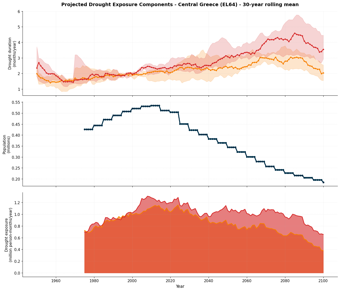
# Visualize projected exposure components
fig, axes = plt.subplots(3, 1, figsize=(14, 12), sharex=True)

# Panel 1: Drought Duration
axes[0].plot(rcp45_stats_rm['year'], rcp45_stats_rm['dmd_median'],
             color='#F77F00', linewidth=2, marker='o', markersize=3)
axes[0].plot(rcp85_stats_rm['year'], rcp85_stats_rm['dmd_median'],
             color='#D62828', linewidth=2, marker='o', markersize=3)
axes[0].set_ylabel('Drought duration\n(months/year)', fontsize=11)
axes[0].set_title('Projected Drought Exposure Components - Central Greece (EL64) - 30-year rolling mean',
                  fontsize=14, fontweight='bold', pad=15)
axes[0].grid(True, alpha=0.3, linestyle='--', linewidth=0.5)
axes[0].spines['top'].set_visible(False)
axes[0].spines['right'].set_visible(False)
# Add uncertainty range
axes[0].fill_between(rcp45_stats['year'],
                rcp45_stats_rm['dmd_p17'],
                rcp45_stats_rm['dmd_p83'],
                color='#F77F00', alpha=0.2, label='RCP4.5 (17th-83rd percentile)')
axes[0].fill_between(rcp85_stats['year'],
                rcp85_stats_rm['dmd_p17'],
                rcp85_stats_rm['dmd_p83'],
                color='#D62828', alpha=0.2, label='RCP8.5 (17th-83rd percentile)')

# Panel 2: Population
axes[1].plot(rcp45_exposure_rm['year'], rcp45_exposure_rm['population']/1e6,
             color='#003049', linewidth=2, marker='s', markersize=3)
axes[1].set_ylabel('Population\n(millions)', fontsize=11)
axes[1].grid(True, alpha=0.3, linestyle='--', linewidth=0.5)
axes[1].spines['top'].set_visible(False)
axes[1].spines['right'].set_visible(False)

# Panel 3: Drought Exposure
axes[2].fill_between(rcp45_stats_rm['year'], 0, rcp45_stats_rm['exposure_median']/1e6,
                     color='#F77F00', alpha=0.6)
axes[2].fill_between(rcp85_stats_rm['year'], 0, rcp85_stats_rm['exposure_median']/1e6,
                     color='#D62828', alpha=0.6)
axes[2].plot(rcp45_stats_rm['year'], rcp45_stats_rm['exposure_median']/1e6,
             color='#F77F00', linewidth=2)
axes[2].plot(rcp85_stats_rm['year'], rcp85_stats_rm['exposure_median']/1e6,
             color='#D62828', linewidth=2)
axes[2].set_ylabel('Drought exposure\n(million person-months/year)', fontsize=11)
axes[2].set_xlabel('Year', fontsize=12)
axes[2].grid(True, alpha=0.3, linestyle='--', linewidth=0.5)
axes[2].spines['top'].set_visible(False)
axes[2].spines['right'].set_visible(False)

plt.tight_layout()
plt.show()
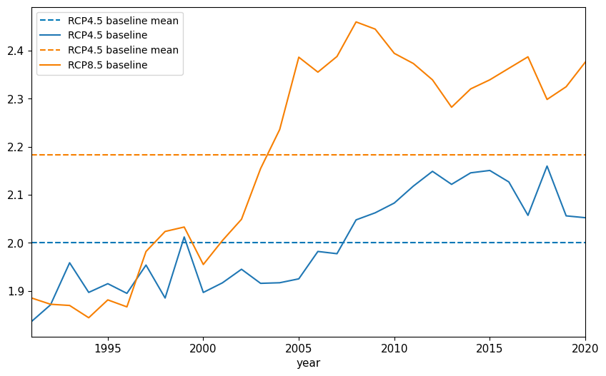
# Calculate anomalies relative to baseline of RCPs
baseline_rcp45 = rcp45_stats_rm[rcp45_stats_rm['year'].between(baseline_start, baseline_end)]
baseline_rcp85 = rcp85_stats_rm[rcp85_stats_rm['year'].between(baseline_start, baseline_end)]
baseline_rcp45_dmd = baseline_rcp45['dmd_median'].mean()
baseline_rcp85_dmd = baseline_rcp85['dmd_median'].mean()
baseline_population = pop_df_filled[pop_df_filled['year'].between(baseline_start, baseline_end)]['population'].mean()
baseline_rcp45_exposure = baseline_rcp45['exposure_median'].mean()
baseline_rcp85_exposure = baseline_rcp85['exposure_median'].mean()

print(baseline_rcp45_dmd)
print(baseline_rcp85_dmd)
print(baseline_population)
print(baseline_rcp45_exposure)
print(baseline_rcp85_exposure)

figure, ax = plt.subplots(figsize=(10, 6))
ax.hlines(baseline_rcp45_dmd, xmin=baseline_start, xmax=baseline_end, color='#0077B6', linestyle='--', label='RCP4.5 baseline mean')
baseline_rcp45.plot(x='year', y='dmd_median', label='RCP4.5 baseline', ax=ax)
ax.hlines(baseline_rcp85_dmd, xmin=baseline_start, xmax=baseline_end, color='#F77F00', linestyle='--', label='RCP4.5 baseline mean')
baseline_rcp85.plot(x='year', y='dmd_median', label='RCP8.5 baseline', ax=ax, color='#F77F00')
ax.set_xlim(1991, 2020)
legend = ax.legend(loc='upper left', fontsize=10, frameon=True)
2.0011656777028186
2.1831219914551876
516921.6624755524
1035118.126941163
1130665.100971916
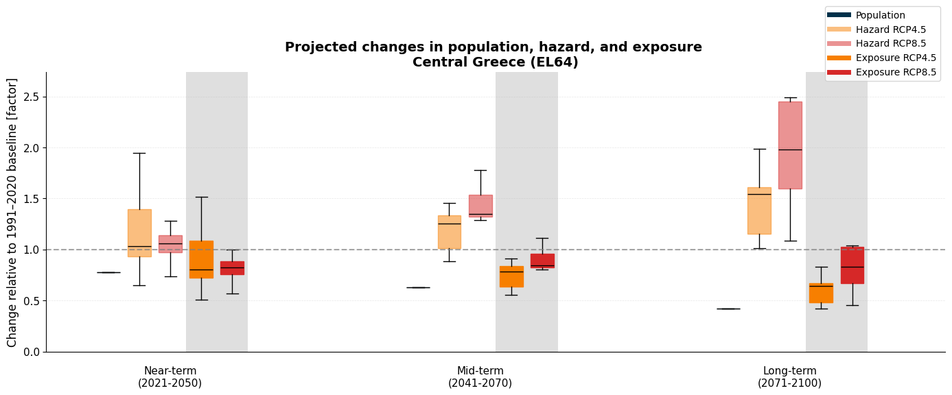
Near-, mid-, and long-term changes
Those timeseries above are nice, but let’s try to get some numbers out of this so that we can communicate a message. Therefore, let’s look at three different time periods:
Near-term future: 2021–2050
Mid-term future: 2041–2070
Long-term future: 2070-2100
Relative changes with respect to baseline period
Further, let’s again evaluate the projections with respect to a baseline period (see best practices outlined in the tutorial assessing changing drought duration under climate change using the WMO recommended baseline period 1991-2020. To facilitate interpretation, we calculate a factorial change of exposure for the region, and we split the exposure into it’s components: relative change of population and drought duration in the near-/mid-/long-term with respect to the baseline period.
# Compute per-model change factors (relative to 1991-2020 baseline) for boxplot
period_order = ['Near-term', 'Mid-term', 'Long-term']


period_info = [
    ('2071-01-01', '2099-12-31', 'Long-term 2071-2100', 0.97),
    ('2041-01-01', '2069-12-31', 'Mid-term 2041-2070', 0.92),
    ('2021-01-01', '2049-12-31', 'Near-term 2021-2050', 0.87)
]
factor_periods = {
    'Near-term': (2021, 2050),
    'Mid-term':  (2041, 2070),
    'Long-term': (2071, 2100),
}

# Baseline: per-model mean dmd over 1991-2020 (averaged across scenarios)
baseline_dmd_models = (
    drought_proj_df[drought_proj_df['year'].between(baseline_start, baseline_end)]
    .groupby(['model', 'scenario'])['dmd'].mean()
    .reset_index()
    .groupby('model')['dmd'].mean()
    .reset_index()
    .rename(columns={'dmd': 'baseline_dmd'})
)

baseline_pop_median = pop_df[
    pop_df['year'].between(baseline_start, baseline_end)
]['population'].median()

period_results = {}

for period_name, (start, end) in factor_periods.items():
    period_pop_median = pop_df[pop_df['year'].between(start, end)]['population'].median()
    population_factor = np.array([period_pop_median / baseline_pop_median])

    hazard_rcp45, hazard_rcp85 = [], []
    exposure_rcp45, exposure_rcp85 = [], []

    for scenario, h_list, e_list in [
        ('RCP4_5', hazard_rcp45, exposure_rcp45),
        ('RCP8_5', hazard_rcp85, exposure_rcp85),
    ]:
        period_dmd = (
            drought_proj_df[
                drought_proj_df['year'].between(start, end) &
                (drought_proj_df['scenario'] == scenario)
            ]
            .groupby('model')['dmd'].mean()
            .reset_index()
            .rename(columns={'dmd': 'period_dmd'})
        )
        m = period_dmd.merge(baseline_dmd_models, on='model')
        m['hazard_factor']   = m['period_dmd'] / m['baseline_dmd']
        m['exposure_factor'] = (m['period_dmd'] * period_pop_median) / (m['baseline_dmd'] * baseline_pop_median)

        h_list.extend(m['hazard_factor'].values)
        e_list.extend(m['exposure_factor'].values)

    period_results[period_name] = {
        'population_factor': population_factor,
        'hazard_rcp45':      np.array(hazard_rcp45),
        'hazard_rcp85':      np.array(hazard_rcp85),
        'exposure_rcp45':    np.array(exposure_rcp45),
        'exposure_rcp85':    np.array(exposure_rcp85),
    }

print("Period results computed:")
for period_name, res in period_results.items():
    print(f"  {period_name}:")
    print(f"    Population factor:        {res['population_factor'][0]:.3f}")
    print(f"    Hazard RCP4.5 (median):   {np.median(res['hazard_rcp45']):.3f}")
    print(f"    Hazard RCP8.5 (median):   {np.median(res['hazard_rcp85']):.3f}")
    print(f"    Exposure RCP4.5 (median): {np.median(res['exposure_rcp45']):.3f}")
    print(f"    Exposure RCP8.5 (median): {np.median(res['exposure_rcp85']):.3f}")
Period results computed:
  Near-term:
    Population factor:        0.779
    Hazard RCP4.5 (median):   1.033
    Hazard RCP8.5 (median):   1.058
    Exposure RCP4.5 (median): 0.805
    Exposure RCP8.5 (median): 0.824
  Mid-term:
    Population factor:        0.626
    Hazard RCP4.5 (median):   1.255
    Hazard RCP8.5 (median):   1.349
    Exposure RCP4.5 (median): 0.785
    Exposure RCP8.5 (median): 0.844
  Long-term:
    Population factor:        0.418
    Hazard RCP4.5 (median):   1.544
    Hazard RCP8.5 (median):   1.982
    Exposure RCP4.5 (median): 0.645
    Exposure RCP8.5 (median): 0.828
# Extended time-series factor boxplots: add exposure factors (RCP4.5 and RCP8.5)
# Population, Hazard RCP4.5, Hazard RCP8.5, Exposure RCP4.5, Exposure RCP8.5

data_to_plot_exp = []
labels_exp = []
box_colors_exp = []

period_info = [
    ('2071-01-01', '2099-12-31', 'Long-term 2071-2100', 0.97),
    ('2041-01-01', '2069-12-31', 'Mid-term 2041-2070', 0.92),
    ('2021-01-01', '2049-12-31', 'Near-term 2021-2050', 0.87)
]

for period_name in period_order:

    res = period_results[period_name]

    data_to_plot_exp.extend([
        res['population_factor'],
        res['hazard_rcp45'],
        res['hazard_rcp85'],
        res['exposure_rcp45'],
        res['exposure_rcp85'],
    ])

    labels_exp.extend([
        f'{period_name}\nPopulation',
        f'{period_name}\nHazard RCP4.5',
        f'{period_name}\nHazard RCP8.5',
        f'{period_name}\nExposure RCP4.5',
        f'{period_name}\nExposure RCP8.5',
    ])

    # Colors: keep population and hazard colored, exposure with grey background

    box_colors_exp.extend([
        '#003049',      # population
        "#F77F00",      # hazard RCP4.5
        '#D62828',      # hazard RCP8.5
        '#F77F00',      # exposure RCP4.5 (grey background)
        '#D62828',      # exposure RCP8.5 (grey background)
    ])

fig, ax = plt.subplots(figsize=(14, 6))

x_positions = [1.1, 1.2, 1.3, 1.4, 1.5, 2.1, 2.2, 2.3, 2.4, 2.5, 3.1, 3.2, 3.3, 3.4, 3.5]
# grey highlighted backgrounds for exposure boxes
# near term: 1.4-1.5, mid term: 2.4-2.5, long term: 3.4-3.5
for x_start in [1.35, 2.35, 3.35]:
    left, bottom, width, height = (x_start, -1, 0.2, 5)
    rect = plt.Rectangle((left, bottom), width, height,
                         facecolor="grey", alpha=0.25)
    ax.add_patch(rect)

bp_exp = ax.boxplot(
    data_to_plot_exp,
    tick_labels=None,
    patch_artist=True,
    widths=0.075,
    showfliers=False,
    boxprops=dict(linewidth=1.0),
    medianprops=dict(color='black', linewidth=1.0),
    whiskerprops=dict(linewidth=1.0),
    capprops=dict(linewidth=1.0),
    positions=x_positions
)
ax.set_xlim(0.9, 3.8)
ax.set_ylim(0, max([max(d) for d in data_to_plot_exp]) * 1.1)
ii=0
for patch, color in zip(bp_exp['boxes'], box_colors_exp):
    patch.set_facecolor(color)
    # use different alpha for exposure boxes to make them look like they are on top of the grey background
    patch.set_alpha(1) if ii in [3, 4, 8, 9, 13, 14] else patch.set_alpha(0.5)
    #patch.set_alpha(0.7)
    patch.set_edgecolor(color)
    ii += 1


# Reference line: no change
ax.axhline(1.0, color='gray', linestyle='--', linewidth=1.5, alpha=0.7)
ax.set_ylabel('Change relative to 1991–2020 baseline [factor]', fontsize=12)
ax.set_title(
    'Projected changes in population, hazard, and exposure \nCentral Greece (EL64)',
    fontsize=14,
    fontweight='bold',
)

ax.grid(True, axis='y', alpha=0.3, linestyle='--', linewidth=0.5)
ax.spines['top'].set_visible(False)
ax.spines['right'].set_visible(False)
# add a legend instead of xticklabels
legend_elements = [
    plt.Line2D([0], [0], color='#003049', lw=5, label='Population'),
    plt.Line2D([0], [0], color='#F77F00', lw=5, alpha=0.5, label='Hazard RCP4.5'),
    plt.Line2D([0], [0], color='#D62828', lw=5, alpha=0.5, label='Hazard RCP8.5'),
    plt.Line2D([0], [0], color='#F77F00', lw=5, alpha=1, label='Exposure RCP4.5'),
    plt.Line2D([0], [0], color='#D62828', lw=5, alpha=1, label='Exposure RCP8.5'),
]
ax.legend(handles=legend_elements, loc='center right', bbox_to_anchor=(1, 1.1), fontsize=10, frameon=True)
# remove x-axis ticks and labels
ax.set_xticks([])
# place x-axis labels manually with rotation at the center of each group just entitled "near-term", "mid-term", "long-term"
ax.text(1.3, -0.25, 'Near-term\n(2021-2050)', ha='center', va='center', fontsize=11)
ax.text(2.3, -0.25, 'Mid-term\n(2041-2070)', ha='center', va='center', fontsize=11)
ax.text(3.3, -0.25, 'Long-term\n(2071-2100)', ha='center', va='center', fontsize=11)
#plt.setp(ax.get_xticklabels(), rotation=25, ha='right')

plt.tight_layout()
plt.show()
End-of-Century exposure
We’ve now seen the factorial change for the near-, mid- and long-term future. Let’s now extract some (absolute) numbers for long-term future.
# Calculate baseline exposure (1991-2020) from climate models
baseline_models = drought_proj_df[
    drought_proj_df['year'].between(baseline_start, baseline_end)
].groupby(['model', 'scenario'])[['year', 'dmd']].median().reset_index()

baseline_pop = pop_df[
    pop_df['year'].between(baseline_start, baseline_end)
]['population'].median()

baseline_models['exposure'] = baseline_models['dmd'] * baseline_pop

# Calculate end-of-century exposure (2071-2100)
eoc_models = drought_proj_df[
    drought_proj_df['year'].between(2071, 2100)
].groupby(['model', 'scenario'])[['year', 'dmd']].median().reset_index()

eoc_pop = pop_df[
    pop_df['year'].between(2071, 2100)
]['population'].median()

eoc_models['exposure'] = eoc_models['dmd'] * eoc_pop

# Merge and calculate changes
changes = eoc_models.merge(baseline_models, on=['model', 'scenario'], suffixes=('_eoc', '_baseline'))
changes['exposure_change'] = changes['exposure_eoc'] - changes['exposure_baseline']
changes['exposure_change_pct'] = (changes['exposure_change'] / changes['exposure_baseline']) * 100

# Summarize by scenario
print("="*80)
print(f"DROUGHT EXPOSURE PROJECTIONS: END-OF-CENTURY (2071-2100)")
print(f"Baseline period: {baseline_start}-{baseline_end}")
print("="*80)

print(f"\nBaseline ({baseline_start}-{baseline_end}):")
print(f"  Population: {baseline_pop/1e6:.2f} million")
baseline_exp = baseline_models.groupby('scenario')['exposure'].median().mean()
print(f"  Drought exposure: {baseline_exp/1e6:.2f} million person-months/year")

print(f"\nEnd-of-century (2071-2100):")
print(f"  Projected population: {eoc_pop/1e6:.2f} million")

for scenario in ['RCP4_5', 'RCP8_5']:
    scenario_changes = changes[changes['scenario'] == scenario]

    exp_median = scenario_changes['exposure_eoc'].median()
    exp_p17 = scenario_changes['exposure_eoc'].quantile(0.17)
    exp_p83 = scenario_changes['exposure_eoc'].quantile(0.83)

    change_median = scenario_changes['exposure_change'].median()
    change_pct_median = scenario_changes['exposure_change_pct'].median()

    n_increase = (scenario_changes['exposure_change'] > 0).sum()
    n_total = len(scenario_changes)

    print(f"\n  {scenario.replace('_', '.')}:")
    print(f"    Median exposure: {exp_median/1e6:.2f} million person-months/year")
    print(f"    Uncertainty range: {exp_p17/1e6:.2f} - {exp_p83/1e6:.2f} million person-months/year")
    print(f"    Change from baseline: {change_median/1e6:+.2f} million person-months/year ({change_pct_median:+.1f}%)")
    print(f"    Model agreement: {n_increase}/{n_total} models show increase")

print("\n" + "="*80)
================================================================================
DROUGHT EXPOSURE PROJECTIONS: END-OF-CENTURY (2071-2100)
Baseline period: 1991-2020
================================================================================
Baseline (1991-2020):
Population: 0.52 million
Drought exposure: 0.89 million person-months/year
End-of-century (2071-2100):
Projected population: 0.22 million
RCP4.5:
Median exposure: 0.54 million person-months/year
Uncertainty range: 0.32 - 0.72 million person-months/year
Change from baseline: -0.33 million person-months/year (-35.2%)
Model agreement: 2/9 models show increase
RCP8.5:
Median exposure: 0.98 million person-months/year
Uncertainty range: 0.73 - 1.12 million person-months/year
Change from baseline: -0.15 million person-months/year (-13.8%)
Model agreement: 4/9 models show increase
================================================================================
Threshold-Based Exposure Analysis
Instead of looking at total drought exposure, we can examine how many people are exposed to significant drought increases over 30-year periods. This approach:
Calculates cumulative drought months for each 30-year period (baseline: 1991-2020, future: 2021-2050, 2041-2070, 2071-2100)
Compares future periods to the baseline to identify drought increases
Evaluates population exposed when increases exceed specific thresholds
Accounts for model uncertainty by showing the range of projections
This helps answer questions like: “How many people will experience at least 10 additional months of drought per 30-year period compared to the 1991-2020 baseline?”
# Configuration: Define 30-year periods and thresholds
period_length = 30  # years per period
thresholds = [10, 15, 20]  # additional drought months per 30-year period

# Define analysis periods
periods = {
    'Baseline': (1991, 2020),
    'Near-term': (2021, 2050),
    'Mid-term': (2041, 2070),
    'Long-term': (2071, 2100)
}

print(f"Configuration:")
print(f"  Period length: {period_length} years")
print(f"  Thresholds: {thresholds} additional drought months per {period_length}-year period")
print(f"\nAnalysis periods:")
for name, (start, end) in periods.items():
    print(f"  {name}: {start}-{end}")
Configuration:
Period length: 30 years
Thresholds: [10, 15, 20] additional drought months per 30-year period
Analysis periods:
Baseline: 1991-2020
Near-term: 2021-2050
Mid-term: 2041-2070
Long-term: 2071-2100
# Calculate cumulative drought months for each 30-year period
def calculate_period_drought_exposure(drought_df, pop_df, periods, thresholds):
    """Calculate population exposed to drought increases per 30-year period.

    Parameters:
    -----------
    drought_df : DataFrame
        Drought projection data
    pop_df : DataFrame
        Population data
    periods : dict
        Dictionary of period names and (start, end) year tuples
    thresholds : list
        List of threshold values for drought month increases

    Returns:
    --------
    dict : Results for each threshold containing exposure statistics by period and scenario
    """

    # Calculate baseline (1991-2020) cumulative drought for each model
    # Note: Take mean across scenarios for historical period (should be identical)
    baseline_start, baseline_end = periods['Baseline']
    baseline_df = drought_df[
        drought_df['year'].between(baseline_start, baseline_end)
    ].groupby(['model', 'scenario']).agg({
        'dmd': 'sum'  # Total drought months over 30 years
    }).reset_index()
    # Average across scenarios (historical period should be same for both RCPs)
    baseline_df = baseline_df.groupby('model')['dmd'].mean().reset_index()
    baseline_df.rename(columns={'dmd': 'baseline_total'}, inplace=True)

    print(f"Baseline cumulative drought ({baseline_start}-{baseline_end}):")
    print(f"  Mean across models: {baseline_df['baseline_total'].mean():.1f} months per {period_length} years")
    print(f"  Range: {baseline_df['baseline_total'].min():.1f} - {baseline_df['baseline_total'].max():.1f} months")
    print(f"  Average per year: {baseline_df['baseline_total'].mean()/period_length:.2f} months/year")

    # Calculate cumulative drought for each future period
    results = {threshold: [] for threshold in thresholds}

    for period_name, (start, end) in periods.items():
        if period_name == 'Baseline':
            continue

        # Calculate total drought months for this period
        period_df = drought_df[
            drought_df['year'].between(start, end)
        ].groupby(['model', 'scenario']).agg({
            'dmd': 'sum'
        }).reset_index()
        period_df.rename(columns={'dmd': 'period_total'}, inplace=True)

        # Merge with baseline (baseline is same for all scenarios)
        merged = period_df.merge(baseline_df[['model', 'baseline_total']],
                                 on='model')
        merged['drought_increase'] = merged['period_total'] - merged['baseline_total']

        # Get population for this period (median across years)
        period_pop = pop_df[pop_df['year'].between(start, end)]['population'].median()

        # For each threshold, calculate exposure
        for threshold in thresholds:
            # Models where drought increase exceeds threshold
            for scenario in merged['scenario'].unique():
                scenario_data = merged[merged['scenario'] == scenario]

                # Count how many models exceed threshold
                exceeds = scenario_data['drought_increase'] >= threshold

                # Population exposed (if any model shows exceedance, all population is at risk)
                # We'll calculate the fraction of models that show exceedance
                exposed_models = exceeds.sum()
                total_models = len(scenario_data)

                # Store results
                results[threshold].append({
                    'period': period_name,
                    'scenario': scenario,
                    'period_years': f'{start}-{end}',
                    'population': period_pop,
                    'exposed_median': period_pop if exposed_models > total_models/2 else 0,
                    'exposed_min': 0 if exposed_models == 0 else period_pop,
                    'exposed_max': period_pop if exposed_models > 0 else 0,
                    'n_models_exceed': exposed_models,
                    'n_models_total': total_models,
                    'drought_increase_median': scenario_data['drought_increase'].median(),
                    'drought_increase_p17': scenario_data['drought_increase'].quantile(0.17),
                    'drought_increase_p83': scenario_data['drought_increase'].quantile(0.83)
                })

    # Convert to DataFrames
    for threshold in thresholds:
        results[threshold] = pd.DataFrame(results[threshold])

    return results

# Calculate exposure for all thresholds
threshold_results = calculate_period_drought_exposure(
    drought_proj_df, pop_df, periods, thresholds
)

print(f"\n✓ Threshold-based exposure calculated for {len(thresholds)} thresholds")
Baseline cumulative drought (1991-2020):
Mean across models: 260.4 months per 30 years
Range: 213.4 - 307.5 months
Average per year: 8.68 months/year
✓ Threshold-based exposure calculated for 3 thresholds
# Visualize drought increase by period with model uncertainty
fig, axes = plt.subplots(1, 2, figsize=(16, 7))

scenarios = ['RCP4_5', 'RCP8_5']
scenario_names = {'RCP4_5': 'RCP4.5 (Moderate Emissions)', 'RCP8_5': 'RCP8.5 (High Emissions)'}
scenario_colors = {'RCP4_5': '#F77F00', 'RCP8_5': '#D62828'}
period_order = ['Near-term', 'Mid-term', 'Long-term']

for idx, scenario in enumerate(scenarios):
    ax = axes[idx]

    # Use the first threshold for the main visualization
    threshold = thresholds[0]
    data = threshold_results[threshold]
    scenario_data = data[data['scenario'] == scenario]

    # Prepare data for plotting
    x_pos = np.arange(len(period_order))
    medians = []
    errors_lower = []
    errors_upper = []

    for period in period_order:
        period_data = scenario_data[scenario_data['period'] == period]
        if len(period_data) > 0:
            median = period_data['drought_increase_median'].values[0]
            p17 = period_data['drought_increase_p17'].values[0]
            p83 = period_data['drought_increase_p83'].values[0]

            # Convert to per-year values for clarity
            medians.append(median / period_length)
            errors_lower.append((median - p17) / period_length)
            errors_upper.append((p83 - median) / period_length)
        else:
            medians.append(0)
            errors_lower.append(0)
            errors_upper.append(0)

    # Create bar chart
    bars = ax.bar(x_pos, medians,
                   color=scenario_colors[scenario], alpha=0.7,
                   edgecolor='black', linewidth=1.5)

    # Add error bars
    ax.errorbar(x_pos, medians,
                yerr=[errors_lower, errors_upper],
                fmt='none', ecolor='black', capsize=8, capthick=2, linewidth=2,
                label='Model uncertainty (17th-83rd percentile)')

    # Add horizontal line at zero
    ax.axhline(0, color='gray', linestyle='--', linewidth=1.5, alpha=0.7)

    # Customize plot
    ax.set_xlabel('Time Period', fontsize=12, fontweight='bold')
    ax.set_ylabel('Drought increase\n(months/year)', fontsize=12, fontweight='bold')
    ax.set_title(scenario_names[scenario], fontsize=13, fontweight='bold', pad=15)
    ax.set_xticks(x_pos)
    ax.set_xticklabels([f'{p}\n({periods[p][0]}-{periods[p][1]})' for p in period_order], fontsize=10)
    ax.legend(loc='upper left', fontsize=10, frameon=True)
    ax.grid(True, alpha=0.3, linestyle='--', linewidth=0.5, axis='y')
    ax.spines['top'].set_visible(False)
    ax.spines['right'].set_visible(False)

    # Add value labels on bars
    for i, (bar, val) in enumerate(zip(bars, medians)):
        height = bar.get_height()
        ax.text(bar.get_x() + bar.get_width()/2., height + errors_upper[i] + 1,
                f'{val:.1f}', ha='center', va='bottom', fontweight='bold', fontsize=10)

plt.tight_layout()
plt.show()

print(f"\n💡 Values show average increase in drought months per year,")
print(f"   relative to baseline period {periods['Baseline'][0]}-{periods['Baseline'][1]}")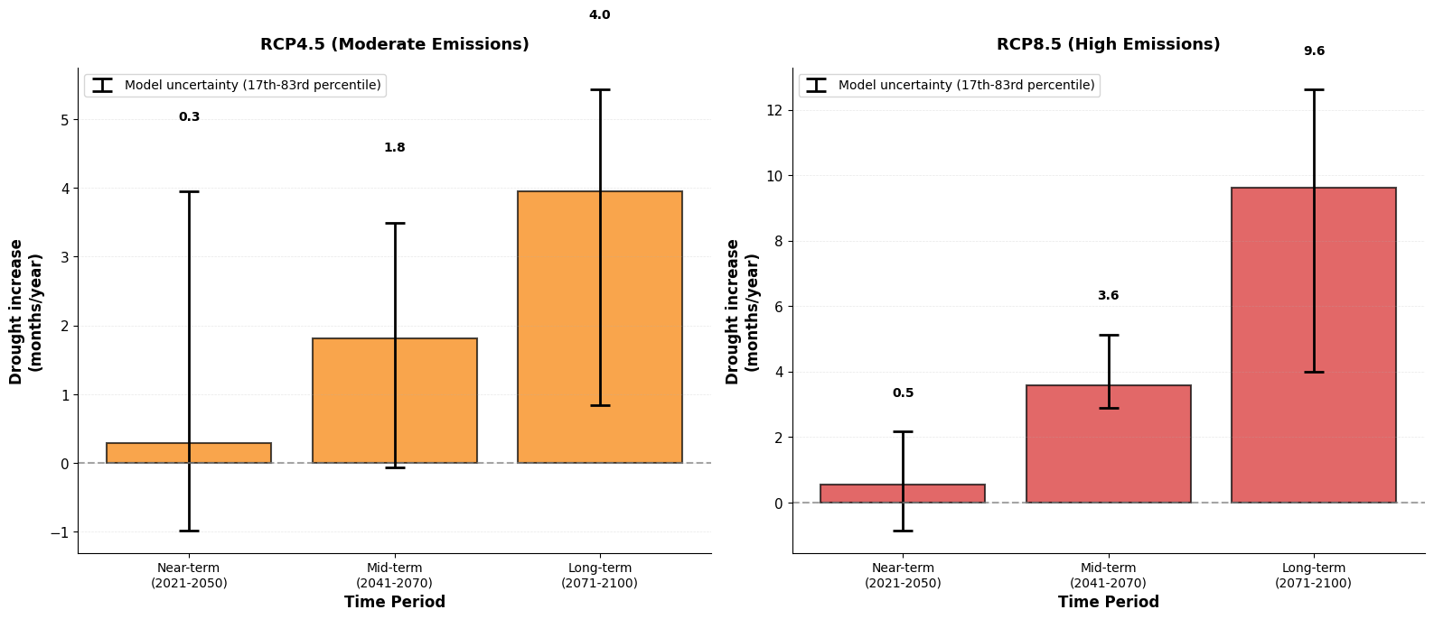
💡 Values show average increase in drought months per year,
   relative to baseline period 1991-2020
# Population exposure when drought increases exceed thresholds
print("="*90)
print(f"POPULATION EXPOSURE TO DROUGHT INCREASES")
print(f"(Baseline: {periods['Baseline'][0]}-{periods['Baseline'][1]})")
print("="*90)

for scenario in scenarios:
    print(f"\n{scenario_names[scenario].upper()}")
    print("-"*90)

    for period in period_order:
        print(f"\n  {period} ({periods[period][0]}-{periods[period][1]}):")

        for threshold in thresholds:
            data = threshold_results[threshold]
            period_data = data[(data['scenario'] == scenario) & (data['period'] == period)]

            if len(period_data) > 0:
                pop = period_data['population'].values[0]
                n_exceed = period_data['n_models_exceed'].values[0]
                n_total = period_data['n_models_total'].values[0]
                pct_models = (n_exceed / n_total) * 100
                drought_increase = period_data['drought_increase_median'].values[0]

                # Estimate population at risk based on model agreement
                if pct_models > 66:  # Strong agreement (>2/3 models)
                    risk_level = "HIGH"
                    pop_at_risk = pop
                elif pct_models > 33:  # Moderate agreement
                    risk_level = "MODERATE"
                    pop_at_risk = pop * 0.5
                else:  # Weak agreement
                    risk_level = "LOW"
                    pop_at_risk = 0

                print(f"    Drought increase ≥ +{threshold} months:")
                print(f"      Model agreement: {n_exceed}/{n_total} models ({pct_models:.0f}%) → Risk: {risk_level}")
                print(f"      Population at risk: {pop_at_risk/1e6:.2f} million ({(pop_at_risk/pop)*100:.0f}% of {pop/1e6:.2f}M)")
                print(f"      Drought increase: {drought_increase:+.1f} months total ({drought_increase/period_length:+.2f} months/year)")

print("\n" + "="*90)
print("\n💡 Interpretation:")
print(f"   - Drought increases show CUMULATIVE additional months over {period_length} years,")
print(f"     relative to {periods['Baseline'][0]}-{periods['Baseline'][1]} baseline")
print(f"   - Example: '+60 months total' = +2.0 months/year average increase")
print(f"   - Population at risk depends on model agreement:")
print(f"     • HIGH (>66% models): All population exposed")
print(f"     • MODERATE (33-66% models): ~50% population exposed")
print(f"     • LOW (<33% models): Minimal exposure")
==========================================================================================
POPULATION EXPOSURE TO DROUGHT INCREASES
(Baseline: 1991-2020)
==========================================================================================
RCP4.5 (MODERATE EMISSIONS)
------------------------------------------------------------------------------------------
Near-term (2021-2050):
Drought increase ≥ +10 months:
Model agreement: 4/9 models (44%) → Risk: MODERATE
Population at risk: 0.20 million (50% of 0.40M)
Drought increase: +8.6 months total (+0.29 months/year)
Drought increase ≥ +15 months:
Model agreement: 4/9 models (44%) → Risk: MODERATE
Population at risk: 0.20 million (50% of 0.40M)
Drought increase: +8.6 months total (+0.29 months/year)
Drought increase ≥ +20 months:
Model agreement: 4/9 models (44%) → Risk: MODERATE
Population at risk: 0.20 million (50% of 0.40M)
Drought increase: +8.6 months total (+0.29 months/year)
Mid-term (2041-2070):
Drought increase ≥ +10 months:
Model agreement: 6/9 models (67%) → Risk: HIGH
Population at risk: 0.32 million (100% of 0.32M)
Drought increase: +54.4 months total (+1.81 months/year)
Drought increase ≥ +15 months:
Model agreement: 6/9 models (67%) → Risk: HIGH
Population at risk: 0.32 million (100% of 0.32M)
Drought increase: +54.4 months total (+1.81 months/year)
Drought increase ≥ +20 months:
Model agreement: 6/9 models (67%) → Risk: HIGH
Population at risk: 0.32 million (100% of 0.32M)
Drought increase: +54.4 months total (+1.81 months/year)
Long-term (2071-2100):
Drought increase ≥ +10 months:
Model agreement: 8/9 models (89%) → Risk: HIGH
Population at risk: 0.22 million (100% of 0.22M)
Drought increase: +118.6 months total (+3.95 months/year)
Drought increase ≥ +15 months:
Model agreement: 8/9 models (89%) → Risk: HIGH
Population at risk: 0.22 million (100% of 0.22M)
Drought increase: +118.6 months total (+3.95 months/year)
Drought increase ≥ +20 months:
Model agreement: 7/9 models (78%) → Risk: HIGH
Population at risk: 0.22 million (100% of 0.22M)
Drought increase: +118.6 months total (+3.95 months/year)
RCP8.5 (HIGH EMISSIONS)
------------------------------------------------------------------------------------------
Near-term (2021-2050):
Drought increase ≥ +10 months:
Model agreement: 5/9 models (56%) → Risk: MODERATE
Population at risk: 0.20 million (50% of 0.40M)
Drought increase: +16.0 months total (+0.53 months/year)
Drought increase ≥ +15 months:
Model agreement: 5/9 models (56%) → Risk: MODERATE
Population at risk: 0.20 million (50% of 0.40M)
Drought increase: +16.0 months total (+0.53 months/year)
Drought increase ≥ +20 months:
Model agreement: 4/9 models (44%) → Risk: MODERATE
Population at risk: 0.20 million (50% of 0.40M)
Drought increase: +16.0 months total (+0.53 months/year)
Mid-term (2041-2070):
Drought increase ≥ +10 months:
Model agreement: 8/9 models (89%) → Risk: HIGH
Population at risk: 0.32 million (100% of 0.32M)
Drought increase: +107.3 months total (+3.58 months/year)
Drought increase ≥ +15 months:
Model agreement: 8/9 models (89%) → Risk: HIGH
Population at risk: 0.32 million (100% of 0.32M)
Drought increase: +107.3 months total (+3.58 months/year)
Drought increase ≥ +20 months:
Model agreement: 8/9 models (89%) → Risk: HIGH
Population at risk: 0.32 million (100% of 0.32M)
Drought increase: +107.3 months total (+3.58 months/year)
Long-term (2071-2100):
Drought increase ≥ +10 months:
Model agreement: 9/9 models (100%) → Risk: HIGH
Population at risk: 0.22 million (100% of 0.22M)
Drought increase: +288.2 months total (+9.61 months/year)
Drought increase ≥ +15 months:
Model agreement: 9/9 models (100%) → Risk: HIGH
Population at risk: 0.22 million (100% of 0.22M)
Drought increase: +288.2 months total (+9.61 months/year)
Drought increase ≥ +20 months:
Model agreement: 8/9 models (89%) → Risk: HIGH
Population at risk: 0.22 million (100% of 0.22M)
Drought increase: +288.2 months total (+9.61 months/year)
==========================================================================================
💡 Interpretation:
- Drought increases show CUMULATIVE additional months over 30 years,
relative to 1991-2020 baseline
- Example: '+60 months total' = +2.0 months/year average increase
- Population at risk depends on model agreement:
• HIGH (>66% models): All population exposed
• MODERATE (33-66% models): ~50% population exposed
• LOW (<33% models): Minimal exposure
Summary
This tutorial demonstrated how to combine drought hazard and population data to estimate drought exposure:
Historical trends:
Historical drought exposure reflects both drought variability and population changes
ERA5 reanalysis provides observed drought patterns
GHS-WUP provides consistent population estimates
Population gaps filled using persistence (forward fill) for complete timeseries
Future projections (2021-2100):
Climate change is projected to increase drought duration
Population changes also affect total exposure
RCP8.5 shows higher exposure than RCP4.5 by end-of-century
Multi-model ensembles quantify projection uncertainty
Threshold-based analysis:
Identifies population exposed to significant drought increases relative to 1991-2020 baseline
Uses cumulative drought months per 30-year period for clearer long-term trends
Provides actionable estimates with model uncertainty quantified via error bars
Accounts for model agreement in assessing exposure risk
Key takeaways:
Exposure = Hazard × Population (both components matter!)
Multiple climate models are essential for assessing uncertainty
Different emission scenarios lead to different exposure outcomes
30-year cumulative analysis reveals long-term trends more clearly than annual values
Model agreement provides confidence levels for risk assessment
Early climate action (RCP4.5) can substantially reduce future drought exposure
Outlook
In the example here, we only have one scenario on how population might change - but this, of course, remains uncertain as well and could/should be incorporated in an exposure assessment. To complete a full drought risk assessment, you would also need to incorporate vulnerability to represent socioeconomic factors that affect drought impacts. Further, having also data on** adaptation, would allow you to evaluate the effectiveness of such measures to reduce exposure or vulnerability.