This short how-to guides you through the steps to create a timeseries of the population using GHS Population data and save it as a csv file. The final csv file can be used as, e.g., exposure data for the drought risk estimation.
We demonstrate the use of two datasets from the Global Human Settlement (GHS) project:
GHS-POP: Historical and projected population (1975-2030), GHS Population Grid. Find more info in Schiavina et al. (2023) and Pesaresi et al. (2024).
GHS-WUP-POP: Urban population projections (1975-2100), GHS WUP Population. Find more info in Schiavina et al. (2025) and Jacobs-Crisioni & others (2025).
Settings
User settings
admin_id = "EL64"  # Example admin ID for Central Greece

# Choose dataset: 'GHS_POP' (1975-2030) or 'GHS_WUP_POP' (1975-2100)
dataset_choice = "GHS_WUP_POP"  # Change to "GHS_WUP_POP" for urban population projections
Setup of environment
import xarray as xr
import numpy as np
import pandas as pd
import matplotlib.pyplot as plt
import geopandas as gpd
import regionmask
from pathlib import Path
import rioxarray as rxr
import os
import re

# Set up data directories
data_dir = Path("../data")
ghs_pop_dir = data_dir / "population" / "GHS_POP"
ghs_wup_dir = data_dir / "population" / "GHS_WUP_POP"

# Set directory and file pattern based on dataset choice
if dataset_choice == "GHS_POP":
    ghs_dir = ghs_pop_dir
    file_pattern = "*/GHS_POP_E*_GLOBE_R2023A_4326_30ss_V1_0.tif"
    dataset_name = "GHS-POP"
    year_range = "(1975-2030)"
elif dataset_choice == "GHS_WUP_POP":
    ghs_dir = ghs_wup_dir
    file_pattern = "*/GHS_WUP_POP_E*_GLOBE_R2025A_4326_30ss_V1_0.tif"
    dataset_name = "GHS-WUP"
    year_range = "(1975-2100)"
else:
    raise ValueError(f"Invalid dataset_choice: {dataset_choice}. Must be 'GHS_POP' or 'GHS_WUP_POP'")

print(f"\nSelected dataset: {dataset_name} {year_range}")
print(f"Data directory: {ghs_dir}")
Selected dataset: GHS-WUP (1975-2100)
Data directory: ../data/population/GHS_WUP_POP
Setup region specifics
# Read NUTS shapefiles
regions_dir = data_dir / 'regions'
nuts_shp = regions_dir / 'NUTS_RG_20M_2024_4326' / 'NUTS_RG_20M_2024_4326.shp'
nuts_gdf = gpd.read_file(nuts_shp)

# Select the region of interest
sel_gdf = nuts_gdf[nuts_gdf['NUTS_ID'] == admin_id]
print(f"Found {admin_id} region: {sel_gdf['NUTS_NAME'].values[0]}")
print(f"Bounding box: {sel_gdf.geometry.total_bounds}")
lon_min, lat_min, lon_max, lat_max = sel_gdf.geometry.total_bounds

# Create a regionmask from the admin region geometry
admin_mask = regionmask.from_geopandas(sel_gdf, names='NUTS_ID')
Found EL64 region: Στερεά Ελλάδα
Bounding box: [21.39637798 37.98898161 24.67199242 39.27219519]
Download Exposure Data
The data is downloaded manually through the following webpage: https://
We download the global data for all years available, but at 30 arcsec resolution, and in the WGS84 (or EPSG: 4326) projection for easier handling of the data afterwards. The images below show the web interface to download the datasets and detail the settings used.
| Download GHS population | Download GHS WUP population |
|---|---|
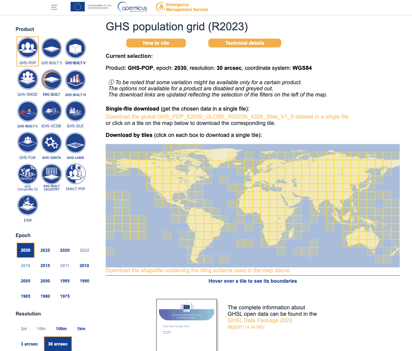 | 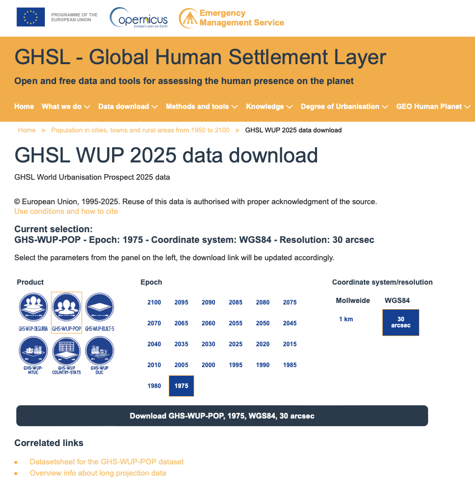 |
GHS-POP (1975-2030): Download files named GHS_POP_E{YYYY}_GLOBE_R2023A_4326_30ss_V1_0.tif for years 1975, 1980, 1985, 1990, 1995, 2000, 2005, 2010, 2015, 2020, 2025, 2030.
GHS-WUP (1975-2100): Download files named GHS_WUP_POP_E{YYYY}_GLOBE_R2025A_4326_30ss_V1_0.tif for years from 1975 to 2100 in 5-year intervals.
Once downloaded, move these files into the following subdirectory structure:
./data/population/GHS_POP/for GHS-POP files./data/population/GHS_WUP_POP/for GHS-WUP files
Process Population Data
Read global data
# List all GHS tif files based on selected dataset
ghs_files = sorted(list(ghs_dir.glob(file_pattern)))
print(f"Found {len(ghs_files)} {dataset_name} files:")
for f in ghs_files:
    print(f"  {f.name}")
Found 26 GHS-WUP files:
GHS_WUP_POP_E1975_GLOBE_R2025A_4326_30ss_V1_0.tif
GHS_WUP_POP_E1980_GLOBE_R2025A_4326_30ss_V1_0.tif
GHS_WUP_POP_E1985_GLOBE_R2025A_4326_30ss_V1_0.tif
GHS_WUP_POP_E1990_GLOBE_R2025A_4326_30ss_V1_0.tif
GHS_WUP_POP_E1995_GLOBE_R2025A_4326_30ss_V1_0.tif
GHS_WUP_POP_E2000_GLOBE_R2025A_4326_30ss_V1_0.tif
GHS_WUP_POP_E2005_GLOBE_R2025A_4326_30ss_V1_0.tif
GHS_WUP_POP_E2010_GLOBE_R2025A_4326_30ss_V1_0.tif
GHS_WUP_POP_E2015_GLOBE_R2025A_4326_30ss_V1_0.tif
GHS_WUP_POP_E2020_GLOBE_R2025A_4326_30ss_V1_0.tif
GHS_WUP_POP_E2025_GLOBE_R2025A_4326_30ss_V1_0.tif
GHS_WUP_POP_E2030_GLOBE_R2025A_4326_30ss_V1_0.tif
GHS_WUP_POP_E2035_GLOBE_R2025A_4326_30ss_V1_0.tif
GHS_WUP_POP_E2040_GLOBE_R2025A_4326_30ss_V1_0.tif
GHS_WUP_POP_E2045_GLOBE_R2025A_4326_30ss_V1_0.tif
GHS_WUP_POP_E2050_GLOBE_R2025A_4326_30ss_V1_0.tif
GHS_WUP_POP_E2055_GLOBE_R2025A_4326_30ss_V1_0.tif
GHS_WUP_POP_E2060_GLOBE_R2025A_4326_30ss_V1_0.tif
GHS_WUP_POP_E2065_GLOBE_R2025A_4326_30ss_V1_0.tif
GHS_WUP_POP_E2070_GLOBE_R2025A_4326_30ss_V1_0.tif
GHS_WUP_POP_E2075_GLOBE_R2025A_4326_30ss_V1_0.tif
GHS_WUP_POP_E2080_GLOBE_R2025A_4326_30ss_V1_0.tif
GHS_WUP_POP_E2085_GLOBE_R2025A_4326_30ss_V1_0.tif
GHS_WUP_POP_E2090_GLOBE_R2025A_4326_30ss_V1_0.tif
GHS_WUP_POP_E2095_GLOBE_R2025A_4326_30ss_V1_0.tif
GHS_WUP_POP_E2100_GLOBE_R2025A_4326_30ss_V1_0.tif
# Read all GHS files and extract years (clipped to region bounding box)
datasets = []
years = []

for tif_file in ghs_files:
    # Read using rioxarray
    ds = rxr.open_rasterio(tif_file)

    # Clip using sel() instead of rio.clip_box to avoid artifacts
    # Note: y coordinates are typically in descending order in raster data
    ds_clipped = ds.sel(
        x=slice(lon_min, lon_max),
        y=slice(lat_max, lat_min)  # Note: reversed for descending y-coords
    )

    # Extract year from filename (looking for pattern E{YYYY})
    year_match = re.search(r'E(\d{4})', tif_file.name)
    if year_match:
        year = int(year_match.group(1))
        years.append(year)
        print(f"Processing year: {year}")
    else:
        print(f"Warning: Could not extract year from {tif_file.name}")
        continue

    datasets.append(ds_clipped)

# Sort datasets and years together by year
sorted_pairs = sorted(zip(years, datasets), key=lambda x: x[0])
years, datasets = zip(*sorted_pairs)

# Concatenate along new time dimension
pop_ds = xr.concat(datasets, dim="time")
pop_ds = pop_ds.rename("population")
pop_ds = pop_ds.squeeze("band", drop=True)

# Assign time based on extracted years
pop_ds["time"] = pd.to_datetime([f"{year}-01-01" for year in years])
pop_ds = pop_ds.assign_coords(time=pop_ds.time)

# Replace potential fill values with NaN (common fill values: -200, -99999, etc.)
pop_ds = pop_ds.where(pop_ds >= 0)

print(f"\n{dataset_name} dataset shape: {pop_ds.shape}")
print(f"Years available: {years}")
print(f"Coordinate ranges: x=[{float(pop_ds.x.min()):.2f}, {float(pop_ds.x.max()):.2f}], y=[{float(pop_ds.y.min()):.2f}, {float(pop_ds.y.max()):.2f}]")
print(f"Data value range: [{float(pop_ds.min()):.2f}, {float(pop_ds.max()):.2f}]")
Processing year: 1975
Processing year: 1980
Processing year: 1985
Processing year: 1990
Processing year: 1995
Processing year: 2000
Processing year: 2005
Processing year: 2010
Processing year: 2015
Processing year: 2020
Processing year: 2025
Processing year: 2030
Processing year: 2035
Processing year: 2040
Processing year: 2045
Processing year: 2050
Processing year: 2055
Processing year: 2060
Processing year: 2065
Processing year: 2070
Processing year: 2075
Processing year: 2080
Processing year: 2085
Processing year: 2090
Processing year: 2095
Processing year: 2100
GHS-WUP dataset shape: (26, 154, 393)
Years available: (1975, 1980, 1985, 1990, 1995, 2000, 2005, 2010, 2015, 2020, 2025, 2030, 2035, 2040, 2045, 2050, 2055, 2060, 2065, 2070, 2075, 2080, 2085, 2090, 2095, 2100)
Coordinate ranges: x=[21.40, 24.67], y=[38.00, 39.27]
Data value range: [0.00, 16747.41]
Extract regional data
# Data is already clipped to bounding box, so we use it directly as pop_region
pop_region = pop_ds

# Create admin region mask
pop_admin_mask_raw = admin_mask.mask(pop_region.x, pop_region.y)
pop_admin_mask = xr.DataArray(
    (~np.isnan(pop_admin_mask_raw.values)).astype(float),
    coords={'y': pop_region.y, 'x': pop_region.x},
    dims=['y', 'x']
)

print(f"{dataset_name} admin mask: {pop_admin_mask.sum().values:.0f} grid cells")
GHS-WUP admin mask: 23973 grid cells
# Diagnostic: Check data quality
print("Data diagnostics:")
print(f"  Population grid shape: {pop_region.shape}")
print(f"  Mask shape: {pop_admin_mask.shape}")
print(f"  Number of masked cells: {pop_admin_mask.sum().values:.0f}")
print(f"  Population data - NaN count: {pop_region.isnull().sum().values}")
print(f"  Population data - Valid values: {(~pop_region.isnull()).sum(['x', 'y']).values}")

# Check a single time slice
sample_time = 0
sample_data = pop_region.isel(time=sample_time)
print(f"\nSample year {pop_region.time.dt.year.values[sample_time]}:")
print(f"  Valid cells (not NaN): {(~sample_data.isnull()).sum().values}")
print(f"  Min value: {float(sample_data.min()):.2f}")
print(f"  Max value: {float(sample_data.max()):.2f}")
print(f"  Mean value: {float(sample_data.mean()):.2f}")
Data diagnostics:
Population grid shape: (26, 154, 393)
Mask shape: (154, 393)
Number of masked cells: 23973
Population data - NaN count: 320892
Population data - Valid values: [48180 48180 48180 48180 48180 48180 48180 48180 48180 48180 48180 48180
48180 48180 48180 48180 48180 48180 48180 48180 48180 48180 48180 48180
48180 48180]
Sample year 1975:
Valid cells (not NaN): 48180
Min value: 0.00
Max value: 15074.26
Mean value: 54.38
Calculate total population
We calculate the total population within the region by summing all population values within the masked area.
# Calculate total population for each year
pop_results = []

for i, year in enumerate(years):
    # Get data for this year
    data = pop_region.isel(time=i)

    # Apply mask and sum population
    masked_data = data.where(pop_admin_mask == 1, 0)
    total_pop = masked_data.sum().values

    pop_results.append({
        'year': year,
        'population': total_pop
    })

    print(f"{year}: {total_pop:,.0f} people")

df_pop = pd.DataFrame(pop_results)
print(f"\n{dataset_name} results:")
print(df_pop)
1975: 425,902 people
1980: 444,018 people
1985: 470,751 people
1990: 490,413 people
1995: 508,224 people
2000: 521,798 people
2005: 531,397 people
2010: 534,820 people
2015: 511,960 people
2020: 505,003 people
2025: 451,386 people
2030: 422,460 people
2035: 402,608 people
2040: 382,952 people
2045: 364,496 people
2050: 344,874 people
2055: 323,530 people
2060: 300,803 people
2065: 279,098 people
2070: 257,720 people
2075: 241,366 people
2080: 226,672 people
2085: 215,900 people
2090: 205,468 people
2095: 195,439 people
2100: 184,935 people
GHS-WUP results:
year population
0 1975 425902.28510579164
1 1980 444017.9732226621
2 1985 470750.8985756294
3 1990 490412.7463494472
4 1995 508224.2765996824
5 2000 521798.0971954223
6 2005 531397.3719865205
7 2010 534819.5705059934
8 2015 511959.95214792923
9 2020 505002.546691046
10 2025 451385.5023026058
11 2030 422459.64027757756
12 2035 402608.38121325243
13 2040 382952.0776415785
14 2045 364495.648229656
15 2050 344873.6430874257
16 2055 323530.45550269866
17 2060 300803.3414491136
18 2065 279097.5541068156
19 2070 257720.00502723106
20 2075 241366.37509886027
21 2080 226671.57679408928
22 2085 215900.20276244936
23 2090 205467.9580282996
24 2095 195438.60577233936
25 2100 184934.71792601293
Save Regional Population Data
Save results to CSV
# Create output directory
output_dir = data_dir / admin_id / "ghs_population"
output_dir.mkdir(parents=True, exist_ok=True)

# Save results with dataset-specific filename
dataset_suffix = "ghs_pop" if dataset_choice == "GHS_POP" else "ghs_wup"
csv_file = output_dir / f"population_{dataset_suffix}_{admin_id}.csv"
df_pop.to_csv(csv_file, index=False)
print(f"Saved {dataset_name} results to: {csv_file}")
Saved GHS-WUP results to: data/EL64/ghs_population/population_ghs_wup_EL64.csv
Output summary
Output files created:
population_ghs_pop_{admin_id}.csv- Population timeseries (1975-2030) from GHS-POPpopulation_ghs_wup_{admin_id}.csv- Population timeseries (1975-2100) from GHS-WUP
These CSV files can now be used as exposure data in drought risk assessments or other analyses.
- Schiavina, M., Freire, S., Carioli, A., & MacManus, K. (2023). GHS-POP R2023A – GHS population grid multitemporal (1975-2030) [Data set]. European Commission, Joint Research Centre (JRC). 10.2905/2FF68A52-5B5B-4A22-8F40-C41DA8332CFE
- Pesaresi, M., Schiavina, M., Politis, P., Freire, S., Krasnodębska, K., Uhl, J. H., Carioli, A., Corbane, C., Dijkstra, L., Florio, P., Friedrich, H. K., Gao, J., Leyk, S., Lu, L., Maffenini, L., Mari-Rivero, I., Melchiorri, M., Syrris, V., Van Den Hoek, J., & Kemper, T. (2024). Advances on the Global Human Settlement Layer by joint assessment of Earth Observation and population survey data. International Journal of Digital Earth, 17(1). 10.1080/17538947.2024.2390454
- Schiavina, M., Freire, S., Carioli, A., MacManus, K., Jacobs-Crisioni, C., Claassens, J., Hilferink, M., & Dijkstra, L. (2025). GHS-WUP-POP R2025A – GHS-WUP population spatial raster dataset, derived from GHS-POP (R2023) and projected using the CRISP model, multitemporal (1975-2100) [Data set]. European Commission, Joint Research Centre (JRC). 10.2905/adba95af-db56-4569-acd3-9513201eba30
- Jacobs-Crisioni, C., & others. (2025). Population projections by degree of urbanisation for the UN World Urbanization Prospects: introducing the CRISP model [Techreport]. Publications Office of the European Union. 10.2760/7163875